Introduction
Overview
Teaching: 30 min
Exercises: 0 minQuestions
Why do we search for long-lived particles?
Why do we use muon detectors?
What signatures are we looking for?
Objectives
Understand the motivation to search for LLPs with muon detectors
Understand the high-multiplicity signature from LLPs due to the unique CMS muon detector design
Have an understanding of the overall analysis strategy and background estimation
We will go through the introductory slides to give you an overview of the motivation to search for LLP with the CMS muon detectors, the analysis strategy, background estimation methods, and limit setting on LLP cross section.
Key Points
Searching for LLPs with the CMS muon detectors that is interleaved with steel return yoke give rise to unique high multiplicity signature that allow us to be sensitive to a broad range of LLP decay modes and to LLP masses below GeV
Long-lived Particles (LLPs)
Overview
Teaching: 10 min
Exercises: 120 minQuestions
What is a long-lived particle?
What is a particle proper decay lengths and lab frame decay lengths?
How often does an LLP decay in the muon detectors?
Objectives
Understand particle lifetime
Reweight LLP lifetime given a signal sample with fixed LLP lifetime
Calculate the geometric acceptance of the endcap muon detector for different LLP lifetimes
After following the instructions in the setup:
cd <YOUR WORKING DIRECTORY>/CMSSW_14_1_0_pre4/src/MDS_CMSDAS
source /cvmfs/sft.cern.ch/lcg/views/LCG_105/x86_64-el9-gcc11-opt/setup.sh
jupyter notebook --no-browser --port=8888 --ip 127.0.0.1
This will open a jupyter notebook tree with various notebooks.
Particle lifetime
Particle decay is a Poisson process, and so the probability that a particle survives for time t (in their own time frame) before decaying is given by an exponential distribution whose time constant depends on the particle’s mean proper decay time($\tau$):
$N(t) = e^{-t/\tau}$
Long-lived particles in CMS are generally considered to have $c\tau$ of ~mm to ~km scale that have non-negligible propability to decay in subdetectors (trackers, calorimeters, and muon detectors), creating displaced signatures.
In this exercise, we will plot the particle proper decay length, from the generator-level LLP information (lab-frame decay vertex and velocity) to verify the exponential behavior.
Open a notebook
For this part, open the notebook called
LLP_lifetimes.ipynband runEx0andEx1to calculate and plot the LLP proper decay length and perform exponential fit.
Discussion 2.1
Are you able to extract the LLP proper decay length from the exponential fit? Does it agree with the expectation?
Particle lifetime reweighting
Since the particle lifetime is usually an unknown parameter. We will interpret our search in a large range of particle lifetimes.
However, to avoid having to generate a large number of signal Monte Carlo samples with different LLP lifetimese, we can reweight the particle lifetime from a signal sample with a given lifetime to a new designated particle lifetime.
For example, we have only generated signal samples with particle lifetimes of 0.1, 1, 10, and 100m, we will use those signal samples to reweight to intermediate particle lifetimes (e.g. 0.5, 5, 50 m)
In this exercise, we will go through how to reweight the particle lifetimes.
Open a notebook
For this part, open the notebook called
LLP_lifetimes.ipynb. RunEx2to reweight the particle lifetimes and plot the proper decay length distribution before and after reweighting to verify the reweighting is done properly.
Discussion 2.2
Why do we reweight from a larger lifetime to a smaller lifetime? What happens when we do the opposite (reweight from smaller lifetime to larger lifetime)?
Probability of LLP decaying in Endcap Muon Detectors
In this section, we will calculate the probability of LLP decaying in the endcap muon detectors for different LLP lifetimes and observe how the probability changes with the lifetime.
Open a notebook
For this part, open the notebook called
LLP_lifetimes.ipynband runEx3
In this exercise, you will first define the geometric decay region of the muon system.
You can find the dimension and layout of the CMS muon system in Fig. 4.1.1 on page 141 of the Muon Detector Technical Design Report
You will calculate the probability of LLP decaying in the endcap muon detectors for LLP mean proper decay lenegths (0.1, 1, 10, 100m) that have been generated.
Then you will call the reweighting function that you’ve written in the previous exercise to calculate the probability, which we call geometric acceptance, for other intermediate proper decay lengths.
Finally, you will plot the geometric acceptance with respect to the LLP mean proper decay lengths.
Discussion 2.3
Do you understand the shape of the geometric acceptance vs. LLP mean proper decay lengths plot?
Why is the peak at 2m, much smaller than the distance between the muon detectors and the interaction point?
Key Points
Particle proper decay lengths follow an exponential decay.
Long-lived particles for LHC searches generally have mean proper decay lengths of ~mm to ~km scale that create displaced signatures in the sub-detectors
LLP lifetime can be reweighted to avoid generating many signal samples with different LLP lifetimes
The probability that an LLP decays in a sub-detector depends on the LLP mean proper decay lengths, so searches for LLPs with different sub-detectors (tracker, calorimeter, and muon detectors) provide complementary coverage to LLPs
MDS Reconstruction
Overview
Teaching: 30 min
Exercises: 180 minQuestions
What is Muon Detector Shower (MDS)?
How are MDS reconstructed?
Objectives
Understand how are MDS reconstructed: the input, the algorithm, the output
Visualize MDS reconstruction
Calculate cluster properties
Calculate MDS reconstruction efficiency with respect to LLP decay position
Ingredient of MDS: Rechits
MDS is a cluster of rechits in the muon system. The main reason for using rechit is that rechit provides sufficient granularity to capture the high-multiplicity nature of the showers coming from LLPs.
What is a rechit?
CSCs consist of arrays of positively-charged anode wires crossed with negatively-charged copper cathode strips within a gas volume.
When muons pass through, they knock electrons off the gas atoms, which flock to the anode wires creating an avalanche of electrons.
Positive ions move away from the wire and towards the copper cathode, also inducing a charge pulse in the strips, at right angles to the wire direction.
Because the strips and the wires are perpendicular, we get two position coordinates for each passing particle.
Figure 3.1
Illustration of a CSC chamber.
Discussion 3.1 :rechits
Can you think of some of the properties of a rechit?
Solution:
The most relevant ones for MDS are: position(x,y,z,eta,phi) and time.
Are there disadvantage/limitation for using rechit as the inputs of MDS?
Solution:
The reconstruction of rechits from the anode/cathode pulses are designed for a single muon, thus it can miss some details about how the shower is developed.
A dedicated machine learning algorithm maybe able to extract those details for even better MDS reconstruction.
Since multiplicity is the most important feature of MDS, the limitation of using rechits is very minimal.
How are CSC chambers arranged?
CSC chambers are arranged into 4 different stations, interleaved with the steel of the flux-return yoke.
Figure 3.2
Illustration of CMS Muon System.
Open a notebook
For this part, open the notebook called
MDS_reconstruction.ipynbto learn how to access and visualize the rechits.
Clustering algorithm
DBSCAN(Density-Based Spatial Clustering of Applications with Noise) is a widely-used, generic clustering algorithm.
It has two parameters, minPts for minimum points to be a cluster and dR for the distance between points.
For clustering MDS, the rechits are the input points and we are clustering in the eta-phi space.
We choose minPts = 50, dR = 0.2. minPts = 50 because it’s more than 2x of the typical number of hits created by a muon in CSC(< 24 hits).
Figure 3.3
Illustration of DBSCAN algorithm. In this diagram, minPts = 4.
Point A and the other red points are core points, because the area surrounding these points in an ε radius contain at least 4 points (including the point itself). Because they are all reachable from one another, they form a single cluster.
Points B and C are not core points, but are reachable from A (via other core points) and thus belong to the cluster as well.
Point N is a noise point that is neither a core point nor directly-reachable.
Cluster properties
Cluster properties are computed from constituent rechits. Here are the descriptions of some key cluster properties:
- Cluster position: average of input rechit positions
- Cluster time: average of input rechit wire time and strip time
- Cluster nStation10: number of stations with at least 10 input rechits in this cluster
- Cluster avgStation10: average station number weighted by number of rechits, using stations with at least 10 input rechits
- Cluster nME11/12: number of rechits coming from ME11 or ME12 in this cluster
Exercise: compute cluster properties
Following the definitions above, complete the function
computeCluster,computeStationPropandcomputeME11_12.
Exercise: plot cluster properties
Plot the cluster properties of background and signal clusters.
To compute for signal clusters,
- run the
DBScanfunctions with signal rechits- store the output in a new variable called
s_cls- add an addition line in
samplesfor plottingTry to read and understand the plotting code as well.
Discussion 3.2: cluster properties
Which variables can be used to distinguish between signal and background?
Solution:
You should be able to see the
N_rechits,time, andME11_12distributions are very different between signal and background.Placing some cuts on these variables should give us separation of signal events from background!
MDS reconstruction efficiency
When an LLP decay in CSC, we want to know
- how often it can make an MDS cluster (this is cluster efficiency) and
- where does the LLP decay when this happens
In this part, we will make a plot of MDS efficiency as a function LLP decay position and try to understand it.
Open a notebook
For this part, continue to the section
MDS reconstruction efficiency for signalto calculate the MDS reconstruction efficiency with respect to the LLP decay position.
Discussion 3.3
Why does the efficiency drops off at the two ends of the muon detectors?
How does the efficiency varies between the muon stations? Do you understand why?
Make a 2D histogram to confirm your understanding!
Key Points
MDS is a cluster of rechits in the muon system, clustered by the DBSCAN algorithm
MDS properties are computed from the input rechits(e.g. position,time & station) and are very powerful of rejecting background
MDS reconstruction efficiency depends on where the LLP decays with respect to the steel, since the decay particles require small amount of steel to initiate the shower and are detected only in the active gas chambers
Analysis Strategy
Overview
Teaching: 15 min
Exercises: 120 minQuestions
What trigger do we use?
What selections do we make to select for signal clusters and reject background clusters?
What are the remaining background compositions for MDS?
Objectives
Understand the background from punch-through jets, muon bremsstrahlung and low pT pileup particles
Understand key variables that are used to remove background and final discriminating variables used to extract signal and estimate background
Benchmark model
The MDS signature is model independent, but to develop an analysis strategy we use the higgs portal as a benchmark model, where the Feynman diagram shown below.
We choose this model because its one of the more difficult model probe at the LHC, with no stable BSM particles to produce large MET and the final state objects from the higgs are generally low pT. This model is also used commonly across many CMS physics searches for sensitivity comparison
Figure 4.1
Feynman diagram of the higgs portal model, where a pair of LLPs (S) are produced from the Higgs and the LLPs can decay to fermions.
Trigger strategy selections
Trigger selection is the beginning of any CMS analysis.
As mentioned in the introductory slides, there’s no dedicated trigger for this signature in Run2.
We are using MET > 200 GeV due to the lack of dedicated trigger on the MDS object.
As a result, in order for signal events to pass the large MET trigger
- the Higgs is recoiled against a high pT jet
- When the LLPs decays beyond calorimeters, the decay
- Since the Higgs has a high pT, the MET will be large
This results in the following event topology for signals:
Figure 4.2
Diagram demonstrating the signal topology. The Higgs is recoiled against an ISR (Initial-State Radiation) jet in a back-to-back configuration. The Higgs decay immediately into 2 LLPs. When LLPs are decaying in the Muon System or beyond, this will result in MET.
Make sure you understand this event topology.
Check your understanding
For this part, open the notebook called
analysis_strategy.ipynbYou will
- confirm that pT of the Higgs matches the size of MET in the event.
- compute the trigger efficiency for signals
The typical trigger efficiency for signals is around 1%
Event selections
The event selections for this search are kept at minimal to be as model independent as possible.
We only apply the MET trigger and an offline MET cut of 200 GeV, due to the use of the high-MET skim dataset.
To select for a signal-like cluster from an LLP, we will investigate a number of variables that are used in the analysis that remove punch-through jet and muon brem background in the following sections.
Cluster-level selections
Open a notebook
For this part, open the notebook called
analysis_strategy.ipynband runEx0to load the ntuples, apply event level selections, and load the relevant branches.
At the cluster-level, we don’t apply any selections for data, while for signal we select clusters that are matched to generator-level LLPs that decay in the muon detectors.
At the event-level, we only apply the MET trigger, offline MET cut, and the required MET filters that are already encoded in the metFilters variable.
Punch-through Jet and Muon Bremsstrahlung Background
The dominant background from the main collision comes from punch-through jets that are not fully contained in the calorimeters and high pT muons that could create bremsstrahlung showers in the muon detectors. To remove those background, we reject clusters by matching them to reconstructed jets and muon.
The pT of the jet/muon that the cluster is matched to are saved in objects called cscRechitClusterJetVetoPt and cscRechitClusterMuonVetoPt.
In this exercise you will plot the two variables for signal and background and apply a selection on the two variables to remove clusters from jets and muons.
Open a notebook
For this part, open the notebook called
analysis_strategy.ipynband runEx1to plot the two variablescscRechitClusterJetVetoPtandcscRechitClusterMuonVetoPt.
Discussion 4.1
Does the shape make sense to you? Why does signal has small values and background has larger values? The analysis apply a cut of
cscRechitClusterJetVetoPt<10andcscRechitClusterMuonVetoPt<20, do you agree with these selections?
Cluster Hits in ME11 and ME12
Additionally, punch-through jets or muon bremsstrahlung showers might not get reconstructed as jets and muons. To fully remove these background, we remove clusters that have hits in the first CSC stations (ME11/ME12) that have little shielding in front.
In this exercise you will plot the number of ME11/ME12 hits in clusters for signal and background and apply a selection on the two variables to remove clusters from jets and muons.
Open a notebook
For this part, open the notebook called
analysis_strategy.ipynband runEx2to plot the number of ME11/ME12 hits in clusters
Discussion 4.2
Does the shape make sense to you? Why does signal has small values and background has larger values? The analysis requires clusters to have no hits in ME11 and ME12, does you agree with the selection?
Cluster $\eta$
After we removed punch-through jets and muon brems, we observed that there are a lot more backgorund in higer $\eta$ region, where the muon reconstruction efficiency is lower and more pileup particles are present to create clusters.
In this exercise you will plot the cluster $\eta$ for signal and background and apply a selection on the variable to remove clusters from high $\eta$ region.
Open a notebook
For this part, open the notebook called
analysis_strategy.ipynband runEx3to plot the cluster $|\eta|$.
Discussion 4.3
Does the shape make sense to you? The analysis requires clusters to have $ | \eta | < 2$, does you agree with the selection?
Cluster time
The remaining background clusters after punch-through jet and muon brem showers from the main collision are removed, are from low pT particles in pileup events. To verify this, you will plot the cluster time for signal and background in this exercise to check for any out-of-time pileup contributions in data.
Open a notebook
For this part, open the notebook called
analysis_strategy.ipynband runEx4to plot the cluster time.
Discussion 4.4
Does the shape make sense to you? Why is data spaced at 25 ns?
Discussion 4.5
Does the data distribution change with and without the vetoes applied? If it does, do you know why?
In the analysis, we apply a selection requiring the cluster time to be between -5 ns and -12.5 ns as the signal region. Additionally, to make use of the out-of-time background clusters, we define a background-enriched early out-of-time (OOT) validation region for the background estimation method used for this analysis, which we will go through in the next episode.
Cluster $N_{\text{hits}}$ and $\Delta\phi\text{(cluster, MET)}$
The final discriminating variables that we will use to extract the signal and estimate background are the number of hits in the cluster ($N_{\text{hits}}$) and the azimuthal angle between the cluster and MET ( $\Delta\phi\text{(cluster, MET)}$). The background estimation method will be described in more detail in the next episode. In this exercise, we will just plot the distributions of the two variables, to understand the shape of the two variables.
Open a notebook
For this part, open the notebook called
analysis_strategy.ipynband runEx5to plot the two variables.
Question 4.1
Why does the $\Delta\phi\text{(cluster, MET)}$ peak at 0 for signal, but flat for background distribution?
Solution 4.1
For signal, the cluster corresponds to the LLP direction and MET corresponds to the higgs direction, so the two objects are aligned as you can see from Figure 4.2.
For background, clusters are produced from underlying events, while MET is calculated from primary event, so the two objects are independent.
Additionally, since $\Delta\phi\text{(cluster, MET)}$ is flat for background, it is also independent to $N_{\text{hits}}$.
This independence is a key property that we will make use of in the next episode to develop the background estimation method.
Discussion 4.7
In the analysis, we apply a selection requiring the $N_{\text{hits}}>130$ and $| \Delta\phi\text{(cluster, MET)}| < 0.75$. Do you agree with the selections?
Now we have defined the set of selections to select signal clusters, next we will go over how to estimate the background yield with a fully data-driven method without using MC simulation.
Key Points
Due to the lack of dedicated trigger, we use the high MET trigger in Run 2 to trigger on the signal
The background from main collision comes from punch-through jet and muon bremsstrahlung and are killed by dedicated jet and muon vetos and active vetos using the first muon detector station
The remaining irreducible background comes from low pT particles from pileup events and clear out-of-time pileup contributions can be observed from cluster time distribution
Two final discriminating variables that are independent for background will be used to extract signal and estimate background
Background Estimation
Overview
Teaching: 20 min
Exercises: 40 minQuestions
What are the source of background for MDS?
How do we estimate the background contribution?
Objectives
Understand background sources for MDS
Understand ABCD method
ABCD method
As you’ve seen in the previous exercise, the main background is from clusters produced in pilup interactions. To estimate the background, we use a fully data-driven background estimation method, the ABCD method, that make use of two independent variables for background: $N_{\text{hits}}$ and $\Delta\phi\text{(cluster, MET)}$.
The ABCD plane is illustrated in Figure 5.1, where bin A is the signal-enhanced region, with large values of $N_{\text{hits}}$ and small values of $\Delta\phi\text{(cluster, MET)}$. The estimation of the number of events in each bin is expressed by:
[\
\begin{align}
N_A &= c_1\times c_2 \times Bkg_C +\mu \times SigA\nonumber
N_B &= c_1\times Bkg_C +\mu \times SigB\nonumber
N_C &= Bkg_C +\mu \times SigC\nonumber
N_D &= c_2\times Bkg_C +\mu \times SigD\nonumber
\end{align}
\]
where:
- SigA, SigB, SigC, SigD are the number of signal events expected in bin A, B, C, and D, taken from the signal MC prediction.
- $\mu$ is the signal strength (the model parameter of interest)
- $c_1$ is the ratio between background in B and C; $c_2$ is the ratio between background in D and C; Both c1 and c2 are essentially interpreted as nuisance parameters that are unconstrained in the fit.
- BkgC is the number of background events in bin C
Figure 5.1
Diagram of the ABCD plane, where bin A is the signal region, $c_1$ is the ratio between background in B and C, and $c_2$ is the ratio between background in D and C.
Validation of the ABCD method
We have shown the previous episode that if the background clusters are from pileup interaction than the two variables $N_{\text{hits}}$ and $\Delta\phi\text{(cluster, MET)}$ should be independent of each other. To validate this assumption and the only background sources are from pileup interactions, we create an out-of-time validation region that is enriched with background and perform ABCD method to check that the prediction from ABCD matches with the observation.
Open a notebook
For this part, open the notebook called
ABCD_validation.ipynband define the OOT control region and perform the validation test by scanning both $N_{\text{hits}}$ and $\Delta\phi\text{(cluster, MET)}$ thresholds.
Discussion 5.1
Does the prediction agree with the observation?
Key Points
The ABCD method requires the use of two independent variables for background, which implies the only source of background should be low pT particles
The method has been validated in the out-of-time validation region, allowing us to proceed to statistical analysis in the signal region
Results and Statistical Analysis
Overview
Teaching: 0 min
Exercises: 180 minQuestions
What is the unblinded result?
How to constrain the ABCD relationship for background in datacards?
Objectives
Understand how to make datacard and constrain the ABCD relationship for background in the datacards
Run Higgs Combine to get Asymptotic limits on BR from the datacards
Produce limit plot with respect to LLP mean proper decay length
Create datacards
Now that we have a well-developed analysis stratey and robus background estimation method, we are ready to produce datacards, look at the unblinded result and perform statistical analysis.
In this exercise, we will walk you through to apply all the signal region selections, add systematic uncertainties and and write the signal and background yield in the ABCD plane to datacards.
Open a notebook
For this part, open the notebook called
create_datacard.ipynbto load the ntuples, apply signal region selection, add systematic uncertainties, and write the signal and background yield in the ABCD plane to datacards.
Discussion 6.1
Do you understand the example datacards? Where is the ABCD relationship constrained for background?
Question 6.1
Do you know what does the rateParam
normdo and why do we add the rateParam to change the normalization of the signal yield?
Solution 6.1
The rateParam in principle can shift the normalization of the signal yield if its allowed to float during the fit. However, we will freeze the rateParam when we run Combine by adding arguments
--freezeParameters norm --setParameters norm=0.001The reason we add a rateParam and scale the signal is because the signal yield varies from O(1) to O(1000) for signals with different LLP lifetimes. However, Combine only works well when the fitted signal strength is between 1 to 15, so we scale the signal yield up/down so that the fitted signal strength fits in that range, and we multiply scale factor back when we plot the limits.
Results
Based on the unblinded data, we can perform a background-only fit to see if the observation agrees with the background prediction.
Run the followiing command to install Higgs Combine:
cd ${CMSSW_BASE}/src
cmsenv
git clone https://github.com/cms-analysis/HiggsAnalysis-CombinedLimit.git HiggsAnalysis/CombinedLimit
cd HiggsAnalysis/CombinedLimit
cd $CMSSW_BASE/src/HiggsAnalysis/CombinedLimit
git fetch origin
git checkout  v10.0.2
scramv1 b clean; scramv1 b # always make a clean build
Choose any of the datacards that you’ve produced and run the following commands:
combine -M MultiDimFit datacard.txt --saveWorkspace -n Snapshot --freezeParameters r,norm --setParameters r=0,norm=0.001

combine -M FitDiagnostics  --snapshotName MultiDimFit --bypassFrequentistFit higgsCombineSnapshot.MultiDimFit.mH120.root --saveNormalizations --saveShapes --saveWithUncertainties
You will get an output file called fitDiagnosticsTest.root.
Open the ROOT file and navigate to the TH1F in shapes_fit_b/chA/total_background by running the following command:
root -l fitDiagnosticsTest.root
shapes_fit_b->cd()
chA->cd()
total_background->GetBinContent(1) # this will print the background prediction
total_background->GetBinError(1) # this will print the uncertainty on the background prediction
Does the background prediction agree with the observation?
Run Higgs Combine to compute limits
To run the Asymptotic frequentist limits we can use the following command (replace test.txt with your datacard path):
combine -M AsymptoticLimits test.txt --freezeParameters norm --setParameters norm=1
# a good rule of thumb for norm is to set it equal to 1./sigA, where sigA is the signal yield in bin A
The program will print the limit on the signal strength r (number of signal events / number of expected signal events) e .g. Observed Limit: r < XXX @ 95% CL , the median expected limit Expected 50.0%: r < XXX, and edges of the 68% and 95% ranges for the expected limits.
The program will also create a ROOT file higgsCombineTest.AsymptoticLimits.mH120.root containing a ROOT tree limit that contains the limit values that we will use later to produce limits plots.
Since we have normalized our signal yield to assume BR(h$\rightarrow$ SS) = 1, the limit on the signal strength r from Combine essentially tells us the limit on BR(h$\rightarrow$ SS), modulo the normalization in signal yield.
Open a script
For this part, open the python script
scripts/run_combine.pyto run over all of the datacards that you produced in the previous exercise and save all the ROOT files in a directory.
- You will have to update the directory of the datacards in the script*
Make limit plots
In this exercise, we will use the limits that were saved in ROOT files produced in the previous exercise to calculate the limit on BR(h $\rightarrow$ SS) with respect to the LLP mean proper decay lengths.
Open a notebook
For this part, open the notebook called
limitPlot.ipynbto plot the expected and observed limits. See if the limit agrees with the one showed on slide 25 of the introduction slides.
Discussion 6.1
Did you expect the shape of the limit to look like this? Why does the sensitivity decreases for very long or very short lifetimes?
Exercise
Now that you have the limit plot for 40 GeV, try to see if you can create datacards, run combine, and make limits plot for 15 and 55 GeV. Try to plot them in the same canvas, like the one in slide 25 of the introduction slide.
Key Points
We can use Higgs Combine to perform statistical analysis and set limits
The value of the limits depend significantly on the LLP mean proper decay length, as the probability of LLP decaying in the muon system strongly correlates with the LLP lifetimes
Event Display (optional)
Overview
Teaching: 0 min
Exercises: 60 minQuestions
How to make event displays of interesting signal simulation?
Objectives
Learn to make event displays by choosing the interesting events in RECO format and open them with cmsShow
In this episode you will create event display of signal simulation events that pass the signal region selectionns
Find and pick events you want to view
We will first find the events that we want to view, by saving the run number, lumi section, and event number of the events in a text file.
Open a notebook
For this part, open the notebook called
event_display.ipynb. This note book is very similar to the notebook in the previous episode, where we make the signal region selection. In addition, we save the run number, lumi section, and event number of the events that we want to view in a text file.
Now run the following code that will pick the ROOT files in the dataset that contain the events that you want based on the run/lumi/event numbers that you supplied:
edmPickEvents.py "/ggH_HToSSTobbbb_MH-125_TuneCP5_13TeV-powheg-pythia8/RunIIFall17DRPremix-PU2017_rp_94X_mc2017_realistic_v11-v1/GEN-SIM-RECO” event_display.txt
The above command will print another command on the screen, like the following, copy and run it in the terminal:
edmCopyPickMerge outputFile=pickevents.root \
  eventsToProcess=1:10122482,1:1055072,1:1055666,1:1127224,1:12138657,1:1441939,1:1441963,1:2514929,1:2896338,1:4255433 \
  inputFiles=/store/mc/RunIIFall17DRPremix/ggH_HToSSTobbbb_MH-125_TuneCP5_13TeV-powheg-pythia8/GEN-SIM-RECO/PU2017_rp_94X_mc2017_realistic_v11-v1/130001/B2A708EC-0D4E-EA11-8B93-0025905C2CBC.root,/store/mc/RunIIFall17DRPremix/ggH_HToSSTobbbb_MH-125_TuneCP5_13TeV-powheg-pythia8/GEN-SIM-RECO/PU2017_rp_94X_mc2017_realistic_v11-v1/130001/84696409-FC4D-EA11-A8CD-0CC47AFF0190.root,/store/mc/RunIIFall17DRPremix/ggH_HToSSTobbbb_MH-125_TuneCP5_13TeV-powheg-pythia8/GEN-SIM-RECO/PU2017_rp_94X_mc2017_realistic_v11-v1/130000/349A8AB2-BF4D-EA11-9AFF-00259073E43C.root,/store/mc/RunIIFall17DRPremix/ggH_HToSSTobbbb_MH-125_TuneCP5_13TeV-powheg-pythia8/GEN-SIM-RECO/PU2017_rp_94X_mc2017_realistic_v11-v1/130001/A4F52ADD-C94D-EA11-B339-7CD30AD091F0.root,/store/mc/RunIIFall17DRPremix/ggH_HToSSTobbbb_MH-125_TuneCP5_13TeV-powheg-pythia8/GEN-SIM-RECO/PU2017_rp_94X_mc2017_realistic_v11-v1/130000/04DB0102-BB4D-EA11-A197-7CD30AD0A78C.root,/store/mc/RunIIFall17DRPremix/ggH_HToSSTobbbb_MH-125_TuneCP5_13TeV-powheg-pythia8/GEN-SIM-RECO/PU2017_rp_94X_mc2017_realistic_v11-v1/130000/D6C63C14-484C-EA11-B04A-1866DA85DC8B.root,/store/mc/RunIIFall17DRPremix/ggH_HToSSTobbbb_MH-125_TuneCP5_13TeV-powheg-pythia8/GEN-SIM-RECO/PU2017_rp_94X_mc2017_realistic_v11-v1/130001/4A6C137D-CA4D-EA11-B475-001E67E7195C.root,/store/mc/RunIIFall17DRPremix/ggH_HToSSTobbbb_MH-125_TuneCP5_13TeV-powheg-pythia8/GEN-SIM-RECO/PU2017_rp_94X_mc2017_realistic_v11-v1/130001/DAD03CA8-624E-EA11-A67F-0242AC1C0504.root
Depending on how many events you’ve chosen, the process might long, don’t choose more than 10 events!
Now you have a ROOT file called pickevents.root that contains the RECO format of the events you have chosen.
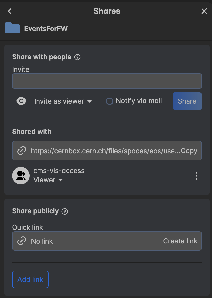
cmsShow is the program used to view event displays. cmsShow is now used with a web-based GUI. Before using the GUI, you need to copy your picked events file to cernbox.
Create a new directory in your personal cernbox. You will need to add viewer access to cms-vis-access
CernBox
Open the events with cmsShow
Once the file is in cernbox and you have given cms-vis-access viewer permission, you can view the event by going to cmsShow
You will now see a graphical interface like this:
Figure 5.1
Event display of a signal event from cmsShow.
By default the csc2DRecHits are not included in the display, go to Add Collectionon the left to add the rechits collections!
Now you can skim through the events that you have selected to see if the clusters appear as you’ve expected.
Key Points
Event displays allow us to view all available collections visually and scrutinize event topologies that are not possible with ntuples